⬅️ Folder: 60.3.7 Economics · Parent: Affordability Crisis · Cross: Health Care · Capitalism · Taxes paid by class
Bottom line
No—not as a general claim about American living standards. A typical American today has far more real income, safer transport and work, better sanitation and climate control, vastly more capable medicine, longer life, lower infant mortality, cheaper food relative to income, and legal opportunities that the 1950s denied to much of the population.
The defensible version of 1950s nostalgia is narrower: housing entry was much cheaper, public college was cheaper, unionized industrial workers had more bargaining power, obesity was rarer, health care consumed less money and administration, and some communities had stronger family and associational stability. Those advantages were real, but they coexisted with smaller and less-equipped homes, worse medicine, higher poverty, dangerous cars and workplaces, heavy smoking and pollution, unpaid domestic labor, legal segregation, and fewer exit options for women and minorities.
Best one-sentence answer: the 1950s made several gateways into adulthood easier for the favored middle class; today makes the contents of life richer, safer, longer, and available to far more people.
The comparison must be symmetrical
Do not compare a 1950s median price with a 2026 premium product, or a 1950s white unionized homeowner with a 2026 population-wide median. Compare like with like:
- Prices relative to incomes, not nominal dollars.
- Equivalent quality, where possible. A 1950 hospital stay, car, house, or telephone is not the same product as its modern counterpart.
- The whole population, not only the group best served by the old rules.
- Outcomes as well as bills. Cheap medicine that cannot save you is not automatically better value.
- Entry versus incumbency. As Affordability Crisis shows, present housing is tolerable for many locked-in owners and punishing for first-time buyers.
Pinker’s Chapter 3 supplement — the 1950s were a crime trough, not the endpoint of a simple trend
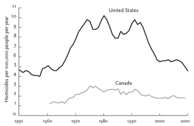
Pinker’s historical series puts the low-crime 1950s inside a sharp U-turn. U.S. homicide rose from 4.0 per 100,000 in 1957 to 10.2 in 1980, then fell to 5.7 in 1999 and 2006 and 4.8 in 2010. Canada remained below one-third of the U.S. rate but moved in parallel: Pinker reports a 0.85 correlation between the national series from 1961–2009 and declines of 35% in Canada versus 42% in the United States during the 1990s.
Figure 3-18 — U.S. homicide, 1950–2010, and Canadian homicide, 1961–2009. The graph strengthens the note’s mixed verdict: the 1950s really were safer than the 1970s–1990s on recorded homicide, but they were not a timeless social baseline, and subsequent decline occurred without restoring the decade’s full family, cultural, or economic settlement. The series ends in 2010 and is not a statement of current rates. Pinker’s cultural “decivilization/recivilization” interpretation remains contested; the Canada comparison also limits any one-country explanation based solely on U.S. incarceration, policing, abortion, demography, or the economy. Chapter 3 synthesis · The rise from 1957 to 1980, PDF pp. 164–166 (file not included in this release) · The 1990s reversal, PDF pp. 176–177 (file not included in this release) · Figure 3-18 and Canada comparison, PDF pp. 177–180 (file not included in this release)
Before saying “the 1950s were better”
The historical comparison strengthens this note’s thesis rather than defeating it. America is vastly richer, safer, healthier, and more comfortable than in 1950: inflation-adjusted disposable personal income per person is about 4.7× as high, while measured real consumption per person is about 4.8× as high; food takes roughly half the income share; life expectancy is about 11 years longer; infant mortality is down about 81%; and amenities such as complete plumbing, air conditioning, safe cars, instant communication, and modern medicine are ordinary rather than rare or nonexistent. These are aggregate-per-person measures, not claims that every family became 4.7× richer; the companion audit defines the measure, checks consumption, and separates averages from the median.
But the nostalgic case contains a real signal: starter housing was much cheaper relative to income, public college cost less, unionized industrial labor had more bargaining power, and family formation followed an easier economic sequence for many households admitted to the postwar compact. Recorded mid-1950s homicide was also low enough that crime should be called mixed, not claimed as an easy modern victory.
Link to originalDefinitions and the poverty-measurement layer: What Poverty Means - Absolute, Relative, and Why Cross-Country Numbers Lie — why cheap manufactured goods and expensive necessities coexist without contradiction, and why a falling price of televisions proves nothing about rent.
The companion note tests economics, the one-income-family claim, lifestyle, crime, basic comforts, medicine, civil rights, and the things the 1950s genuinely did better. Its conclusion: the 1950s made several gateways into adulthood easier for the favored middle class; today makes the contents of life richer, safer, longer, and open to far more people. The policy goal is to recover postwar entry affordability and social infrastructure without recovering exclusion, inferior medicine, or lower material living standards.
The scoreboard
| Domain | What the 1950s case gets right | What defeats the broad nostalgia claim | Verdict |
|---|---|---|---|
| Income and consumption | A single industrial wage could support a modest household in many places; wage growth was broadly shared | Real disposable income per person was $11,306 in 1950 vs $52,689 in 2025 (2017 dollars), about 4.7× as high now | Today, decisively |
| Poverty and unemployment | Postwar labor markets were tight in 1951–53 and wage growth was broadly shared | Official poverty fell 22.4% → 10.6%, and fewer Americans were poor in 2024 than in 1959 despite the population nearly doubling; unemployment was higher in 1958–59 than today | Today, decisively |
| Housing | Purchase prices were much lower relative to income; new suburbs expanded supply rapidly | Homes were smaller and less equipped; only 55% were owner-occupied in 1950 vs about 65% now; access was racially exclusionary | 1950s for entry price; today for quality and access |
| Food and goods | Some durable goods were repairable and expectations were lower | Food absorbed 22.1% of disposable income in 1949; the current ERS series puts it near 9.7% in 2025 | Today |
| Basic comforts | Less digital clutter; simpler products | About one-quarter of homes lacked an indoor flush toilet, only 12% had a TV, and air conditioning was rare; 88% of households used AC by 2020 | Today, decisively |
| Health care | Much cheaper; less billing and insurance bureaucracy | Life expectancy rose from roughly 68 years to 79; infant mortality fell from 29.2 to 5.53 per 1,000; modern care treats conditions that were death sentences | Today for outcomes; 1950s for price simplicity |
| Crime | Recorded homicide was low: 5.4 per 100,000 in 1950, roughly the neighborhood of the current rate | Modern long-run victimization measures start later; domestic and sexual violence were less visible and differently defined; today is far safer than the 1980s–90s | Mixed; no clean win |
| Transport and safety | Less congestion and fewer miles exposed to traffic | The traffic-death rate is around one-sixth its 1950 level per mile; modern cars have restraints, crash structures, airbags, and emergency response | Today |
| Work and bargaining | Union density peaked near 28–34% in the mid-1950s; industrial workers had more leverage and defined benefits | Work was more dangerous, dirtier, more physical, and occupational access was openly restricted by race and sex | 1950s for bargaining; today for safety and access |
| Family and community | Earlier marriage, more two-parent households, denser civic and religious participation in many places | Some stability reflected economic dependence, discrimination, stigma, and inability to exit abusive or unhappy arrangements | A real but morally mixed advantage |
| Civil freedom and opportunity | The era had strong local institutions for those admitted to them | Legal segregation, sex-specific job ads, housing discrimination, and unequal education were normal; the major federal protections came in 1964–74 | Today, decisively |
1. Economics: cheaper houses did not mean a richer society
Real resources are much greater now—but “4.7×” needs a careful definition
The cleanest broad measure is not the sticker price of a hamburger or a house. It is real disposable personal income per person: an estimate of the after-tax income available to people for spending or saving, adjusted for inflation and divided by the population.
| Year | Real disposable personal income per person (2017 dollars) |
|---|---|
| 1950 | $11,306 |
| 2025 | $52,689 |
| Change | +366%, or 4.66× |
Source: BEA series via FRED, A229RX0A048NBEA, updated May 28, 2026. BEA defines disposable personal income as personal income minus personal current taxes; “real” means deflated with the Personal Consumption Expenditures price index. BEA definition · real-DPI definition.
What the arithmetic actually says
That is a 366% increase, not a 466% increase: the modern level equals the original 100% plus 366% more. Spread across 75 years, it is approximately 2.1% real growth per person per year, compounding to a doubling about every 34 years.
The dollar labels are chained 2017 dollars, not literal 1950 or 2025 cash. BEA uses a chain-weighted quantity index so changing relative prices and consumption patterns do not freeze the calculation to a 1950 shopping basket. The useful information is the 4.66 ratio and growth rate; $52,689 should not be read as a claim that the average person received that sum in cash or could buy exactly $52,689 of a fixed 2017 basket.
What is inside “disposable personal income”
This is broader than wages. It includes income received by or on behalf of people from:
- wages and salaries, including employer supplements such as pension and insurance contributions;
- proprietors’ and rental income;
- interest and dividends; and
- government transfers such as Social Security and other benefits;
then subtracts personal current taxes. It does not include unrealized or realized capital gains as personal income. “After tax” is also narrower than ordinary speech: BEA subtracts items such as income and personal-property taxes, but not sales taxes, which are reflected in market prices rather than deducted in the DPI account. BEA personal-income definition · BEA tax FAQ.
So “real resources” is shorthand for the inflation-adjusted command over market goods and services that the personal-income accounts allocate per resident after personal current taxes. It is a powerful broad prosperity indicator—not a complete welfare measure.
A cross-check: people really do consume about 4.8× more per person
One might object that income merely accumulated at the top and never became ordinary consumption. BEA’s separate real personal consumption expenditure per capita series provides a useful check. Averaging its quarterly annualized observations:
| Measure (chained 2017 dollars per person) | 1950 | 2025 | Ratio |
|---|---|---|---|
| Real disposable personal income | $11,306 | $52,689 | 4.66× |
| Real personal consumption expenditures | ≈$10,107 | ≈$48,284 | ≈4.78× |
The consumption measure counts goods and services purchased by or on behalf of households. It therefore includes third-party-paid consumption, such as employer- or government-financed medical care, not merely what a family pays at the register. BEA/FRED real PCE per capita, A794RX0Q048SBEA · BEA definitions.
This corroboration matters: it says the 4.7× result is not only an accounting claim about available income. The economy supplies roughly 4.8 times the real volume of measured personal consumption per resident. Some of that is additional quantity—more travel, appliances, housing space, education and medical treatment—and some is quality improvement captured imperfectly by the price indexes.
What 4.7× does—and does not—prove
What it establishes
- The United States is not generally producing or consuming at a 1950 material level.
- Population growth and ordinary inflation do not explain the increase; the series already divides by population and removes price changes.
- A story based only on a cheap 1950 house or hamburger mistakes one relative price for the economy-wide standard of living.
- The result is consistent with the concrete gains elsewhere in this note: lower food burden, more complete plumbing and climate control, safer travel, more education and vastly more capable medicine.
What it does not establish
- Not “the median person is 4.7× richer.” This is total DPI divided by total population, so an unequal gain at the top raises the average. It needs a median-income check.
- Not “every household has 4.7× the money.” Household size fell, paid work moved into markets, and family/household definitions changed.
- Not “discretionary cash is 4.7× higher.” Employer-paid health benefits, transfers, rent imputation and other non-paycheck items enter personal income; costly necessities can absorb the gain.
- Not “welfare or happiness is 4.7× higher.” The measure omits leisure, household production, community, autonomy, environmental quality, crime, family stability and subjective wellbeing.
- Not “every modern price is more affordable.” Housing entry, college, child care and some health costs can worsen relative to income even while total real resources rise.
- Not a clean measure of technological value. Free digital services and entirely new products are hard to price, while greater medical spending may represent valuable treatment, high unit prices, administrative waste, or all three.
The median-family check gives a smaller—but still large—gain
The 1950 Census reported median family income of $3,073 in 1949 dollars. Its own historical comparison puts 2019 median family income at $80,944 in 2019 dollars; inflation-adjusting the 1949 figure yields only about $32,000–$33,000 in 2019 purchasing power. Definitions and household composition changed, so this is directional rather than an exact growth rate. It still contradicts the claim that the median family was generally richer then. See the Census Bureau’s 1950 Census facts.
That implies a rough median-family increase of about 2.5×, well below the 4.7× per-capita aggregate. Several forces create the gap: income inequality, smaller families, more earners per family, transfer and asset income, employer-provided benefits, and differences between the CPI conversion used in the Census comparison and BEA’s PCE-deflated national-account series.
The debate-safe formulation
The economy’s inflation-adjusted after-tax personal income per resident is about 4.7 times its 1950 level, and measured real consumption per resident is about 4.8 times as high. That proves an enormous increase in average material resources, not an equal 4.7-fold gain for every family. A rough median-family comparison is closer to 2.5 times, while particular gateways—especially buying a first home—can still be less affordable today.
The single-income household is often misdescribed
The familiar picture—one wage, detached house, car, stay-at-home wife, several children—was real for a large and culturally central group. But four corrections matter:
- It was not the population-wide norm of effortless abundance. In 1950, the Census counted roughly 10 million of 40 million families below $2,000 in annual money income. The official poverty series begins in 1959, when 22.4% of people were poor; it was 10.6% in 2024. The measure has limitations, but mass poverty was not invented recently. Census historical poverty tables · 2024 report.
- The household bought less because it produced more at home. The non-employed spouse supplied child care, cooking, cleaning, sewing, shopping, elder care, and administrative work without a market wage. Calling this a one-income lifestyle can hide a two-worker household in which only one worker was paid.
- The consumption bundle was smaller. One smaller home, often one car, one bathroom, no central air, few appliances, no paid child care, limited travel, and little purchased entertainment is cheaper than the bundle now treated as middle class.
- The bargain was not equally open. Housing covenants, segregated schools, discrimination in lending and employment, and sex-segregated occupations allocated the best version of this model selectively.
Food is the clearest anti-nostalgia price
In 1949, families and individuals spent 22.1% of disposable personal income on food, including 18.0% at home. The live USDA series used in Affordability Crisis places total food near 9.7% in 2025. Even after the post-2020 grocery shock, food requires less than half the income share it did around 1950. USDA historical review, table 22 · current ERS interactive series.
That improvement is easy to miss because modern households buy more restaurant food and prepared food. Nostalgia often compares 1950 home-cooked staples plus unpaid preparation time to today’s mixed bundle of groceries, restaurants, delivery, and convenience.
Housing is the strongest exception
The 1950 median home value was $7,354; median family income was $3,073, a rough value-to-income ratio of 2.4×. The modern ratio is around 5× in Affordability Crisis, and the payment gap is worse because mortgage rates rose while prices stayed high.
That is a genuine deterioration in entry affordability. Do not wave it away with larger kitchens or better insulation. A young family cannot live inside a quality adjustment; it must qualify for the payment.
But the full comparison adds three facts:
- Homeownership was lower, not higher: about 55% in 1950, versus 65.0% in Q2 2026. Census historical note · current Housing Vacancy Survey.
- The product improved: modern houses are generally larger, have more bathrooms, better electrical capacity, insulation, climate control, kitchens, fire protection, and accessibility.
- The cheap pathway was exclusionary: Brown v. Board was not decided until 1954; most housing discrimination was not federally outlawed until the Fair Housing Act of 1968. National Archives on Brown · HUD history.
Correct housing conclusion
The 1950s did housing supply and entry price better, while rationing access and tolerating lower quality. The policy lesson is to recover rapid building and attainable starter homes—not the discrimination, segregation, or one-size-fits-all household model that accompanied them.
2. Lifestyle: less choice can look like less stress
The 1950s case often shifts from purchasing power to the texture of life: slower pace, more neighbors, stable families, less screen addiction, clearer norms. Some of this is real. It is also hard to compare because it mixes facts with values.
What likely felt better
- Less constant digital interruption, algorithmic comparison, and surveillance.
- More routine face-to-face contact through churches, unions, clubs, neighborhoods, and extended families.
- A clearer and earlier sequence into adulthood: job, marriage, starter home, children.
- Less choice overload and fewer recurring bills.
- More children roaming locally and more adults embedded in stable institutions.
What the postcard omits
- Conformity had an enforcement mechanism. Divorce, nonmarital birth, homosexuality, religious dissent, disability, mental illness, interracial relationships, and gender nonconformity carried legal or severe social penalties.
- Stability is not the same as wellbeing. Lower divorce can mean better marriages, but it can also mean financial dependence, stigma, weak legal protection, and no safe exit.
- The unpaid-work burden was gendered. A simpler consumer bundle often required more cooking, cleaning, laundry, mending, and caregiving.
- The neighborhood was not open to everyone. A cohesive suburb produced by restrictive covenants and discriminatory lending cannot be counted as pure social capital.
- Private suffering was less legible. Domestic violence, marital rape, child abuse, sexual assault, and workplace harassment were less likely to be named, reported, or prosecuted under modern definitions.
The fair conclusion is not that community was an illusion. It is that community and constraint were bundled together. Modern America gained autonomy and exit options but often failed to build voluntary institutions strong enough to replace what compulsory norms once supplied.
3. Crime: the nostalgic side has a partial point
This category should not be argued with a fake statistic. The 1950s were not the high-crime 1970s–90s.
What can be compared
The CDC’s age-adjusted homicide series reports:
| Year | Homicide deaths per 100,000 |
|---|---|
| 1950 | 5.4 |
| 1955 | 4.8 |
| 1960 | 5.2 |
| 1973 | 10.5 |
Source: CDC, Homicide Trends in the United States, 1900–1974. Coding standards and age adjustment changed, so use the source’s own series rather than mixing it casually with FBI counts.
The best current evidence shows reported violent crime fell 4.5% in 2024, with murder down 14.9% from 2023. BJS estimates a 370.8 violent-offense rate per 100,000 in 2024, down from 393.9, while the victimization survey shows violent victimization far below 1993. FBI 2024 release · BJS 2024 reported-crime estimates · NCVS.
What cannot be honestly claimed
- There is no consistent national victimization survey for 1950; NCVS begins in 1973.
- Definitions of rape, domestic violence, child abuse, hate crime, and police reporting changed radically.
- Recorded crime reflects both offending and the willingness/capacity to report it.
- A national rate hides enormous differences by neighborhood, race, age, and sex.
Debate-safe crime conclusion
The 1950s probably were safer than the late 1960s through 1990s on homicide, and some mid-1950s years may have been modestly safer than today. That does not establish a general superior lifestyle. Current violence is far below the 1990s peak, while many forms of family and sexual violence are more visible and more broadly criminalized now. Call this category mixed, not a modern landslide.
Everyday safety outside crime is much better now
Crime is only one risk of leaving home. In 2024, the traffic fatality rate was estimated at 1.20 deaths per 100 million vehicle-miles, versus 7.24 in 1950—roughly six times as dangerous per mile. Modern roads are imperfect and cars are faster and more numerous, but seat belts, airbags, crash engineering, child restraints, trauma medicine, and drunk-driving enforcement changed the stakes. FHWA historical table FI-200 · NHTSA 2024 estimate.
3b. Poverty and unemployment: the two rows the scoreboard was missing
Added 2026-08-22. Definitions, measurement caveats, and the international comparison live in What Poverty Means - Absolute, Relative, and Why Cross-Country Numbers Lie.
The headline series
| Measure | Late 1950s | Recent |
|---|---|---|
| Official poverty rate | 22.4% (1959) | 10.6% (2024) |
| People officially poor | 39.5 million | 35.9 million |
| U.S. population | ~177 million | ~340 million |
| Unemployment | 5.5% (1959) | 4.1% (July 2026) |
| Real GDP per capita | $19,296 (Q4 1959) | $70,812 (Q2 2026) |
The number that does the work
Not the rate — the absolute count. The U.S. population nearly doubled between 1959 and 2024, and fewer people were counted as poor at the end of that period than at the start. This is the single hardest fact for a total-decline narrative to absorb.
But note where the gain came from. Almost all of the decline happened in one decade: 22.4% in 1959 → 12.1% in 1969. Since then the rate has oscillated with the business cycle in a band of roughly 10–15% rather than continuing to fall. Anyone arguing continuous progress on poverty is overclaiming; the honest claim is a large one-time level shift that has since held.
| Year | Official poverty rate |
|---|---|
| 1959 | 22.4% |
| 1969 | 12.1% |
| 1979 | 11.6% |
| 1989 | 12.8% |
| 1999 | 11.9% |
| 2009 | 14.3% |
| 2019 | 10.5% |
| 2024 | 10.6% |
Unemployment was not uniformly low in the 1950s
| Year | Unemployment |
|---|---|
| 1950 | 5.3% |
| 1951 | 3.3% |
| 1952 | 3.0% |
| 1953 | 2.9% |
| 1954 | 5.5% |
| 1955 | 4.4% |
| 1956 | 4.1% |
| 1957 | 4.3% |
| 1958 | 6.8% |
| 1959 | 5.5% |
| July 2026 | 4.1% |
Today’s rate is roughly ordinary by 1950s standards — worse than the exceptionally tight labor markets of 1952–53, clearly better than 1958–59. The 2025 annual average was 4.3%; July 2026 represents about 6.9 million unemployed people.
The structural caveat that stops this being a clean win
Identical unemployment rates do not describe identical labor markets. In 1950 roughly 29% of working-age women participated in the labor force; by 2019 it was 59%. The denominator, the household structure behind it, and the meaning of a single-earner household all changed. This connects directly to The single-income household is often misdescribed.
One measurement conflict to disclose when using these
The OPM (10.6%) ignores noncash benefits and tax credits, which understates progress. The SPM (12.9% for 2024) counts them but also subtracts medical and childcare costs, and comes out higher. Cite whichever you like, but say which — and note that the SPM figure is currently provisional pending a Census revision announced 17 July 2026.
4. Basic comforts: the ordinary 1950 home was not the television set
The 1950 Census counted 45.98 million dwellings. Among them:
- About 11 million—nearly one-quarter—reported an outside/other toilet or no flush toilet.
- Only about 73% had access to a bathtub or shower.
- 94% had electric lights.
- 80.2% had mechanical refrigeration.
- Only 12% had a television.
- Coal remained the most commonly reported heating fuel among heated homes.
Source: Census Bureau, 1950 Census housing facts.
The correct lesson is not that everyone lived primitively. Electricity, radio, refrigerators, telephones, automobiles, and indoor plumbing had already transformed life. The lesson is that amenities now considered below the floor were still unevenly distributed, and the modern bundle had barely begun.
By 2020, 88% of U.S. households used air conditioning, including two-thirds using central AC or a central heat pump; 99% had a refrigerator. EIA on air conditioning · EIA on home electricity uses.
Add the non-housing comforts that a price index struggles to value:
- instant long-distance communication and navigation;
- a global library, news archive, music catalog, and video-call system in one pocket device;
- safer food storage and a much broader year-round food supply;
- automatic laundry and dishwashing;
- rapid emergency communication;
- quieter, cleaner, more reliable cars with heating and cooling;
- disability access, hearing aids, corrective procedures, and assistive technology;
- cheap computing, photography, translation, and entertainment.
Do not turn this into “people cannot complain”
A smartphone does not compensate a renter for being unable to buy a home. Cheap electronics and expensive land can coexist. The point is to reject a total-collapse story, not to deny the concentrated entry crisis documented in Affordability Crisis.
5. Health care: more expensive, but not the same product
The 1950s advantage was real
Health spending absorbed 4.4% of national output in 1950, compared with 18.0% in 2024. Billing was simpler, insurance less pervasive, administrative overhead lower, and families were less exposed to today’s premiums, deductibles, prior authorization, opaque networks, and surprise prices. CMS long-run historical table · current CMS National Health Expenditure data.
That is a serious modern failure. A richer country should not need the world’s most labyrinthine payment system.
But the medical product was radically worse
| Outcome | 1950 | Latest comparable figure | Change |
|---|---|---|---|
| Life expectancy at birth | about 68.2 years | 79.0 years (2024) | +10.8 years |
| Infant mortality | 29.2 per 1,000 births | 5.525 per 1,000 (2024) | −81% |
| Paralytic polio | >21,000 cases at the 1952 peak | no U.S.-origin wild-polio case since 1979 | effectively eliminated domestically |
Sources: CDC Vital Statistics 1950 · CDC Mortality in the United States, 2024 · CDC Pink Book, polio.
The aggregate gains understate what changed. In 1950 there was no modern intensive care, organ transplantation, CT or MRI, coronary bypass, statins, minimally invasive surgery, neonatal intensive care, routine dialysis, effective combination chemotherapy for many cancers, modern antiretroviral treatment, or today’s anesthesiology and trauma systems. Many congenital conditions, infections, heart attacks, premature births, and cancers that are survivable now were untreatable.
Why sticker-price comparisons mislead
A 1950 hospital sold fewer tests, fewer drugs, fewer specialists, fewer interventions, and fewer years of survival. Calling it “the same care at a lower price” is like comparing the fare for a propeller flight with a modern jet while ignoring speed, safety, and reach.
That does not excuse every modern dollar. It separates two questions:
- How much of the spending buys real capability and longer life? A substantial amount.
- How much reflects high prices, administrative waste, monopoly power, defensive medicine, and bad incentives? Also substantial.
The right target is modern outcomes with less rent extraction and bureaucracy, not 1950 expenditure with 1950 medicine. See also Health Care and the current-cost audit in Affordability Crisis > Q1 — What is actually rising, and by how much?.
6. Better for whom? The exclusion problem
Any population-wide claim must count people whom the nostalgic picture leaves outside the frame.
- In 1954, Brown v. Board held state-school segregation unconstitutional; seventeen states still required segregated schools and four permitted it. National Archives.
- The Civil Rights Act of 1964 outlawed segregation in public accommodations and employment discrimination based on race, color, religion, sex, or national origin. Its necessity is evidence about the world immediately before it. National Archives.
- The Fair Housing Act of 1968 outlawed most housing discrimination; sex protection was added in 1974 and disability/familial status in 1988. HUD.
- The Equal Credit Opportunity Act was not enacted until 1974. CFPB.
- Before Title VII, employers openly segregated job classifications, and newspaper ads routinely separated jobs for men and women. EEOC history.
These are not decorative caveats. They change the denominator. A system that offers a superb pathway to a selected group and blocks others cannot be judged solely by the selected group’s mortgage payment.
The decisive question
Would you accept the 1950s bargain without knowing your race, sex, sexuality, disability status, family background, health condition, or whether your marriage would be safe?
7. What really was better in the 1950s?
1. Starter-home affordability and housing production
This is the strongest case. Land and homes cost far less relative to family income, the country built at the metropolitan fringe at enormous scale, and first-time buyers did not face today’s combination of a high price-to-income ratio and high mortgage rates. Quality and exclusion caveats do not erase the entry-price advantage.
What to recover: abundant small homes, legal multifamily housing, faster permitting, serviced land, infrastructure expansion, and lower transaction costs.
2. Public higher-education prices
Comparable national series become firmer around 1959–60, not 1950. They show public four-year tuition and total charges consuming a much smaller share of family income than they later did. Present net tuition has improved from its 2010s peak, as Affordability Crisis notes, but the long-run increase and debt-financed pathway remain real. NCES historical college-cost series.
What to recover: lower instructional and administrative costs, strong public subsidy tied to completion, and credible non-college routes into skilled work.
3. Worker bargaining power for organized industrial labor
Depending on denominator and series, union density peaked around 28–34% in the mid-1950s, compared with 10.0% in 2025. Collective bargaining more often delivered wage scales, pensions, health benefits, paid leave, seniority rules, and a voice at work. BLS historical discussion · BLS 2025 union rate · CRS series and comparability warning.
This advantage was uneven: many unions excluded or marginalized Black workers and women; agriculture, domestic work, and much of the South sat outside the protected core; industrial jobs could be dangerous and authoritarian.
What to recover: bargaining power, wage compression, portable benefits, and worker voice without closed racial/sex hierarchies or requiring everyone to work in a factory.
4. Lower obesity and more routine physical activity
The earliest nationally measured series is 1960–62, when adult obesity for ages 20–74 was 13.4%, versus roughly 40% today. Daily life involved more walking and physical labor, less ultra-processed food, and less screen time. CDC historical obesity series.
But the health environment was not generally superior: smoking was pervasive, lead and air pollution were worse, cars and workplaces were more dangerous, and medicine was less capable. Treat lower obesity as a real advantage, not proof of overall better health.
What to recover: walkable communities, routine movement, healthier food defaults, active childhood, and less screen dependence.
5. Lower medical-system cost and administrative burden
Health care used a far smaller share of income and GDP, and there was less insurance bureaucracy. This is a genuine advantage even after acknowledging that the product was less capable.
What to recover: transparent prices, fewer intermediaries, simpler payment, competitive supply, and administrative standardization—while preserving modern treatment.
6. Some forms of social cohesion and a clearer path to adulthood
Marriage happened earlier; civic, religious, union, and neighborhood institutions were denser in many communities; and adult milestones were less delayed. These can be goods. The evidence is less clean than for prices or mortality, and causation is disputed.
What to recover: voluntary association, third places, family-friendly housing and work, local participation, and time for relationships—without coercive conformity or trapping people in bad families.
7. A few crime measures
Recorded homicide in the mid-1950s was low, sometimes slightly below plausible present rates. Acknowledge this. It strengthens the rest of the argument by removing an indefensible talking point.
What to recover: effective local order, informal guardianship, competent policing, and low violence—while retaining modern recognition of domestic, sexual, and hate crimes.
8. Why the nostalgia remains persuasive
The selected-survivor effect
People remember the families that secured the house, pension, and stable neighborhood. They less often remember households in substandard rural housing, segregated neighborhoods, institutions, unsafe marriages, dangerous jobs, or early graves.
The age effect
People comparing their childhood with adulthood compare a period when someone else paid the bills with a period when they do. Personal responsibility rises even if living standards do too.
The visible-price effect
A 1950 house price is legible. The value of a 10.8-year gain in life expectancy, a fivefold reduction in infant mortality, instant emergency communication, safer anesthesia, or an eliminated disease is not posted on a shelf.
The gateway-versus-bundle effect
Modern life gives far more inside the bundle but charges more for the gateways—housing, child care, health insurance, and credentialing. Those gateways determine whether young adults can form households. A person can rationally say “society is richer” and “my route into adulthood is worse” at the same time.
The distribution effect
Aggregate prosperity does not guarantee that a specific worker, renter, region, or generation receives it. The broad claim “America is poorer than in 1955” is false; the narrower claim “some entrants face worse prices than comparable earlier entrants” can be true.
9. Debate kit
| Claim | Short answer | Concession that keeps it honest |
|---|---|---|
| ”One income supported a whole family.” | Often by buying a smaller bundle and relying on a second adult’s unpaid labor; average real DPI is about 4.7× and real consumption about 4.8× their 1950 levels. | Housing entry really was easier; the rough median-family gain is closer to 2.5× than 4.7×. |
| ”A house cost only $7,000.” | Income was about $3,000; compare ratios, quality, interest, and access. The 1950 ratio was still much better. | Today’s first-time-buyer payment is a genuine crisis. |
| ”Food and goods were affordable.” | Food took about 22% of disposable income around 1950 versus roughly 10% now. | Modern convenience spending is optional only up to a point when all adults work. |
| ”Crime was lower.” | Homicide was low in the 1950s; concede it. But long-run victimization data do not extend that far and many private crimes were underrecognized. | Some mid-1950s homicide rates may indeed beat today’s. |
| ”Health care was cheap.” | Yes—and it could do much less. Infant mortality was five times higher and life expectancy about eleven years shorter. | Modern U.S. prices and administration remain indefensibly high. |
| ”Families were stronger.” | Some were; some were simply harder to leave. Stability, freedom, and wellbeing must be measured separately. | Modern atomization and delayed family formation are real losses. |
| ”People had fewer things but were happier.” | Possible for some, but happiness surveys are not directly comparable and the claim is normative. | More consumption does not automatically create meaning or belonging. |
| ”Everything is unaffordable now.” | Goods, food, communication, and many comforts are historically cheap; the crisis is concentrated in entry to housing and a few services. | Concentrated costs can still block the life people want. |
The strongest closing
Do not defend every feature of the present. Say: “The 1950s solved some gateways better—especially starter housing, bargaining power, and an earlier family path. But it delivered a smaller, riskier, shorter life under rules that excluded millions. The goal is to combine 1950s entry affordability and social infrastructure with modern medicine, safety, comfort, and equal citizenship.”
10. What this comparison should change in the affordability debate
The comparison redirects policy away from nostalgia and toward mechanisms:
- Build the missing starter homes. The 1950s housing advantage was fundamentally a supply and financing achievement, although distributed unjustly.
- Attack health-care prices and administration without pretending old medicine was adequate. Preserve capability; remove rents and friction.
- Lower the cost of family formation. Housing, child care, predictable work, and time matter more than making televisions cheaper.
- Rebuild bargaining power and non-college career ladders. The old industrial compact cannot simply be restored, but its wage-setting function can be replaced.
- Design for voluntary community. Third places, walkability, local institutions, and family-sized housing can produce connection without enforcing 1950s conformity.
- Measure entry separately from averages. A society can be richer in aggregate while treating new buyers, renters, and parents worse.
This is the bridge to Affordability Crisis: today is not a general collapse in living standards. It is a rich society with a severe bottleneck in a few life-defining gateways.
Method and evidence limits
- “The 1950s” is a decade, not a point. This note uses 1950 where possible and 1959–62 where national series begin. Every table names the year.
- Household definitions changed. Family, household, per-capita, and tax-unit income are not interchangeable.
- Quality adjustment is necessary but contestable. It is strongest for medicine, cars, appliances, and communication; less persuasive when a buyer simply cannot qualify for a starter home.
- Crime categories changed. Homicide is the best long-run anchor; use rape, assault, and domestic-violence comparisons cautiously.
- Civil-rights law is not the same as lived equality. Modern discrimination persists. The point is that the old exclusion was both more explicit and more legally supported.
- Current figures are dated. Income is 2025, mortality 2024, housing Q2 2026, and AC 2020. Update before publication.
- National averages hide group experience. Race, sex, class, geography, age, disability, and homeownership status can reverse a national conclusion.
Core sources
Income, consumption, poverty, and food — BEA/FRED real disposable income per capita · BEA/FRED real consumption per capita · BEA definitions and statistical conventions · Census 1950 facts · Census 1950 family-income report · Census historical poverty tables · USDA Food Cost Review 1950–97 · USDA current Food Expenditure Series
Housing and comforts — Census 1950 housing facts · 1950 homeownership benchmark · Census Housing Vacancy Survey · EIA 2020 air conditioning · EIA home electricity uses
Health and safety — CDC Vital Statistics 1950 · CDC Mortality 2024 · CDC polio history · CMS 1950–90 long-run table · current CMS National Health Expenditure data · FHWA traffic fatalities 1900–2024 · NHTSA 2024 traffic estimate · CDC obesity history
Crime — CDC homicide trends 1900–74 · FBI reported crime 2024 · BJS Crime Known to Law Enforcement 2024 · BJS National Crime Victimization Survey
Rights, work, and education — National Archives: Brown v. Board · National Archives: Civil Rights Act · HUD history · EEOC legal history · CFPB on ECOA · BLS mid-century labor history · CRS union-density history · NCES historical college costs
Handwritten Notebook Pages
Source
Open Were the 1950s better than today? notebook pages — start at notebook p. 144 (file not included in this release).